An Introduction To Genetic Algorithms
I had some time this weekend and discovered the magic that is pandoc, so I decided to convert the chapter on Genetic Algorithms over to my blog for easier reading. There may be some odd formatting due to the conversion, and my quick hand fixes. Please keep in mind that this introduction was in the context of a longer document, but I think it still provides some useful concepts and examples.
Introduction
As early as the 1950s scientists were looking at how evolution could be used to optimize solutions in engineering and scientific problems [Mitchel (1998)]. John Holland at the University of Michigan [Holland (1975)] began working and publishing on the idea of Genetic Algorithms in particular over 30 years ago. Genetic Algorithms, GA, are a way to automate the optimization process based on techniques used in biological evolution. GA can be compared to other optimization techniques like hill climbing or simulated annealing, in that these techniques all try to find optimal solutions to problems in a generic enough way that they can be applied to a large range of problem types.
GA is generally implemented using the following high level steps:
-
Determine a way to encode solutions to your problem, the encoding will be used to define the chromosomes for your Genetic Algorithm.
-
Determine a way to score your solutions. We will call this scoring mechanism the fitness function.
-
Run the Genetic Algorithm using your encoding and scoring to find a “best" solution. In the next few sections we will see how GA generates new individuals to score.
The individual elements of a chromosome will be called genes to match the biological terminology.
A Sample Problem: The Shortest Path
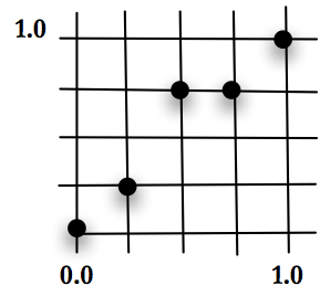
Let’s look at an example of the first two high level steps for applying GA. Imagine the X-Y plane, with the unit square between 0.0 and 1.0 in each direction. Place a point at (0.0,0.0) and another at (1.0,1.0). These are the lower-left and upper-right corners. Create a grid of squares by breaking the remaining X and Y space into equal length sections. Our problem is to place points at intersections of the grid, pictured in Figure below, one for each X value, that when connected makes the shortest line. In other words, minimize the distance between a set of points where the first and last point are in a fixed position and the X value of the points is pre-determined. Keep in mind that the possible values for X and Y are discrete based on the grid.
The answer for this problem can be determined in many ways. The question will be, can GA find the solution. As we explore GA with this problem, it is worth noting that GA may not be the best technique to solve it. This is ideal for a test problem, since it allows us to appreciate how GA is performing compared to other techniques. This problem also offers an interesting framework because changing one point at a time, as hill climbing or a steepest descent technique would try to do, won’t necessarily work; moving one point might create a longer section between it and its neighbors. For an algorithm to optimize the solution, it may be necessary for all of the values in the encoding to move toward the best answer at the same time. The solution space is non-trivial.
Encoding the Shortest Path Problem
We will encode the shortest path problem onto a discrete grid using a constant called \(\psi\), and the following steps:
-
Break the X-axis and Y-axis from 0 to 1.0 into \(\psi\) sections.
-
Store the Y-value at each X point, excluding the two ends, as a single integer from 0 to \(\psi\)
The first point is always (0.0,0.0) and last point is always (1.0,1.0) and are not stored in the chromosome. For example, the chromosome:
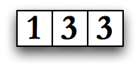
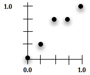
will translate into the set of points:
Because we are going to fix the first and last point to the two corners, we will have a total of \(\psi - 1\) integers for each chromosome. This insures that we can scale this problem for MGGA by splitting each X value in half. The value of \(\psi\) is also used to split the X and Y axis equally so that scaling during MGGA, discussed in the next section, will be equal in both directions.
This is a pretty simple problem and encoding. But imagine that we use \(\psi = 128\) This would result in a problem space with \(127\) X’s, each with \(129\) possible values, or \(129^{127} = 1.1 \times 10^{268}\) possible encodings. That is a huge search space.
Scoring the Shortest Path Problem
To score each individual we use a fitness function that performs the following steps:
-
Calculate the X value for each point by dividing the X axis into \(\psi\) parts, keeping in mind that the first element of the chromosome is at \(0.0\) and the last at \(1.0\). In Figure [fig:images~xa~nd~y~] with \(\psi = 4\) the X values will be \(0\), \(0.25\), \(0.5\), \(0.75\) and \(1.0\).
-
Treat the value for each X location as \(\psi\) units that add up to a height of \(1.0\), so if \(\psi = 4\) the Y values will range from \(0\) to \(4\), corresponding to values of \(0\), \(0.25\), \(0.5\), \(0.75\) and \(1.0\).
-
Calculate the length of the line connecting all of the points by adding up the distance between the points defined by consecutive genes, looping and summing until all of the gene pairs are mapped onto line segments and included.
-
Subtract the result from \(1.0\) to make \(1.0\) the best fitness and all others less than \(1.0\). The value of \(1.0\) is not achievable, since the distance is always greater than \(0\). However, I use this convention throughout this dissertation to provide a consistent value for the best possible fitness.
Put simply the fitness for a chromosome is:
\[\begin{split} F(x) = 1 - \text{sum of length of line segments} \ = 1 - \sum_{i=0}^\psi \sqrt[2]{(x_{i+1}-x_i)^{2} + (y_{i+1}-y_i)^{2}} \end{split} \label{eq:sample_problem_fitness}\]
Given a problem encoding and fitness function, lets look at the Genetic Algorithm itself.
The Genetic Algorithm
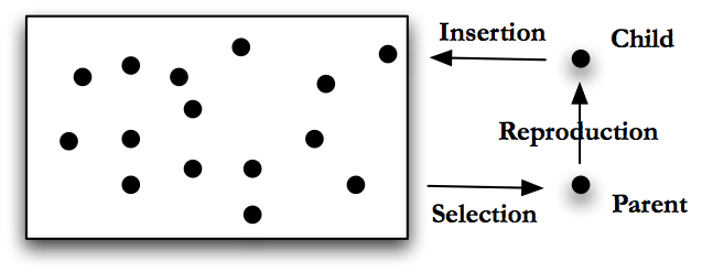
Genetic algorithms are generally run in one of two modes: steady state or generational, [Langon and Poli (2002) page 9]. In steady state GA the program will perform the following steps, pictured in Fig. Steady State GA.
-
Generate a number of possible solutions to the problem. Encode these solutions using an appropriate format. This group of encoded solutions is called a population.
-
Score the individuals in the population using the fitness function.
-
Use some sort of selection mechanism, see Section Selection Mechanics, to pull out good individuals, call these individuals parents.
-
Build new solutions from the parents using GA operations, see Section Genetic Operations. Call these new individuals children, and this process reproduction.
-
Insert the children into the population, either by replacing their parents, by growing the population or by replacing some other set of individuals chosen using a selection mechanism.
-
Return to step 2. (In steady state GA, the population remains basically the same, or steady, we just replace or add to it.)
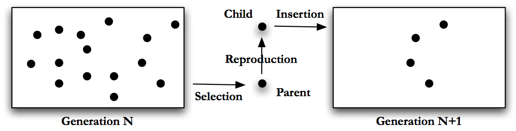
Generational GA changes the last step in this algorithm. In generational GA the algorithm will perform the following steps, pictured in Fig. Generational GA.
-
Generate a number of possible solutions to the problem, encode these solutions using an appropriate format. This group of solutions is called a population or generation.
-
Score the individuals in the population using the fitness function.
-
Use some sort of selection mechanism, see Section Selection mechanics, to pull out good individuals, we will use these as parents.
-
Build new solutions from the parents using GA operations, see Section Genetic Operations. Call these new individuals the children and this process reproduction.
-
Insert the children into a new population. (Note - in generational GA we make a new population each time, in steady state GA we reused the same population.)
-
Repeat generating children until the new population is full.
-
Return to step 2, with the new population as the current population.
The genetic algorithm will loop until it meets some termination condition. Termination conditions include: a sufficiently good individual is found, some number of individuals have been tested, or a fixed amount of computing time is used. Generational GA includes an additional termination condition of running until a specific number of generations are executed.
For this dissertation I have used generational GA exclusively because it is the most like other optimization techniques. Also, generational GA fit well into a batch processing model that runs on the available clusters at the University of Michigan.
Diversity
As in biology, GA has to worry about available genetic material. The concept of available material is called diversity. In GA, diversity is a measure of how much of the problem space the current population represents, [Eiben and Smith (2003) page 20]. In our sample problem, if all of the individuals had a zero for the first gene, this would represent less diversity than if some individuals have a one in the first gene. Diversity can be thought of as a measure of the available genetic material. In order to truly search a problem space, we want to have as much viable genetic material as possible.
Perhaps the main implication of good diversity is the ability to avoid local minimum and maximum in a problem space, [Tomassini (2005) page 37]. GA has a number of ways to keep and indeed improve diversity in the population. These will be discussed in the sections below.
Selection Mechanisms
One of the key steps in the “Genetic Algorithm" is selecting parents for the next generation. Selection is one of the main ways to maintain diversity in a population. The selection process can be handled a number of ways.
Random Selection
Random selection is the process of picking individuals from the population with no concern for their fitness. This selection scheme keeps a lot of diversity, but doesn’t help move the algorithm toward a solution. Random selection can suffer from the side effect that it loses good individuals to bad luck, simply because they are not randomly picked.
Top Selection
Top selection takes the fitness for every individual in a population and ranks them. Then the highest scoring individual is used as the parent for every child. Always selecting the top individual makes very little sense in generational GA, but can make some sense in steady state GA. If we use top section for generational GA we would be creating a new population with a single parent. As we will see in the next few sections, the only way to change that parent will be mutation. So with top selection we would essentially be performing an inefficient hill climbing optimization. With steady state GA, we would still be essentially hill climbing, but without completely replacing the population each time.
Truncation Selection
Truncation selection also ranks the individuals by fitness, but instead of always picking the top scoring individual, truncation selection randomly picks individuals from the top \(N\%\) of individuals. If \(N\) is small, only the very top individuals are picked. If \(N = 100\%\), truncation selection becomes random selection.
Truncation selection has a small cost in the ranking process. Depending on population size this can be an issue. But the more important issue with truncation selection is that it removes “bad" individuals from the population. This is a concern because sometimes, the bad individuals are holding useful genetic material. In our shortest path sample problem, a bad individual might be the only one with a one in the first gene. By always killing lower fitness individuals, truncation selection can hurt the long term success of the population.
Roulette, or Fitness Proportional Selection
Roulette selection tries to solve the problem of reduced diversity associated with losing bad individuals by randomly choosing from all individuals, [Banzhal et al. (1998) page 130]. However, unlike random selection where every individual has an equal chance to be picked, roulette selection uses the fitness of each individual to give more fit individuals a higher probability of being picked. To achieve this, roulette assigns a selection probability for each individual based on its fitness, as follows:
-
Calculates the sum across all fitness scores.
\[S = \sum_{i=0} f_i \text{, where \(f_i\) is the fitness for individual \(i\)} \label{eq:roulette_fitness}\]
-
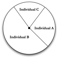
Assign each individual a probability based on its fitness divided by the sum of all fitness scores, see Fig. Roulette Selection.
\[p_i = f_i / S \label{eq:roulette_prob}\]
-
Spin the wheel to get a number \(r\) between \(0\) and \(1\).
-
Walk the list of individuals, from the first one in the population to the last, adding each individuals probability to the running total:
\[s_j = \sum_{i=0}^{r} p_i\text{.} \label{eq:roulette_sum}\]
-
Stop when the value on the wheel falls in an individual’s probability zone,
\[s_{j-1} < r \le s_j \text{, select individual \(j\).} \label{eq:roulette_eq}\]
Roulette selection won’t necessarily lose “bad" individuals, and has only a small overhead. Roulette selection also puts selective pressure on the Genetic Algorithm by giving good individuals a better chance to be used for reproduction. However, it does suffer from the ability for a very fit individual to drown out a number of worse individuals. For example, given a population of 10 individuals, if one has a fitness of \(1.0\) and the rest have a fitness of \(0.1\), the higher scoring individual will be selected about \(\frac{1}{2}\) of the time. This, like rank and truncation selection, can hurt diversity in a population.
Rank Selection
There is another version of Roulette selection, sometimes called Rank Selection, that uses the individual’s rank, rather than its raw fitness to assign a probability. This selection method removes the chance for a single individual, or small group of individuals, to dominate the fitness wheel, [Eiben and Smith (2003) page 60]. Rank selection reduces the chance of keeping a “bad" individual with “good" genes.
Tournament Selection
Tournament selection [Eiben and Smith (2003) page 63] tries to solve the problem of choosing good individuals at the cost of diversity in a novel way. In tournament selection we chose a tournament size, call it \(TS\). In its simple form, each time an individual needs to be selected for reproduction, a small tournament is run by:
-
Randomly pick \(TS\) individuals
-
Take the highest scoring individual from this group
This algorithm uses random selection to get the members of the tournament, so good and bad scoring individuals are equally likely to make it into a tournament. Unfortunately, in this simple form, tournament selection will leave zero chance for the worst individual to be used for reproduction, since it can’t win a tournament. This leads to a modified algorithm:
-
Pick a percentage of times we want the worst individual to win the tournament. This value, \(PW\), can be tuned. A low value of \(PW\) will keep bad individuals out, while a high value can increase diversity by allowing more bad individuals in.
-
Pick \(TS\) individuals
-
Randomly pick a number between \(0\) and \(100\).
-
If the number is greater than \(PW\) take the highest scoring individual from this group, otherwise take the lowest scoring individual in the group
A useful feature of tournament selection for GA users is that it has two tuning mechanisms, the size of the tournament and the chance that bad individuals win. Tournament selection is good for diversity, since it allows bad individuals to win in a controllable way. By changing tournament size it is possible to make tournament selection more like random selection, using a small tournament, or more like truncation selection, by using a large tournament.
Because of these nice features, all of the GA done in later chapters will use tournament selection. The tournament sizes will be 4 or 5 individuals. Based on experiments these values allow close to \(98\%\) of each population to participate in at least one tournament. The \(PW\) for my runs will generally be \(25\%\). The value of \(25\%\) was based on an initial desire to allow lower scoring individuals to win tournaments without overwhelming good individuals. In places where my runs suffer from diversity issues, a possible direction for future work will be to try different values for this tuning parameter.
Selection and Fitness Function Requirements
The choice of fitness function and selection mechanism are connected. Suppose that you have the choice of two fitness functions. Both rank properly, in that the better individuals have higher fitnesses. But one is smooth and the other is discontinuous or lumpy. What I mean by lumpy is that the fitness function likes to group individuals around certain scores, and if individuals improve they might jump to another group of scores.
Given these two choices of fitness function, which is best? To answer that really depends on the selection algorithm. If you use roulette selection, then lumpy or discontinuous fitness functions could be bad because they would give larger probabilities to an individual that is near a discontinuity in the fitness function, even if the difference between that individual and one on the other side of the discontinuity is ultimately minimal. On the other hand, rank selection or tournament selection won’t have this problem because they use the ordering of fitness scores rather than the raw fitness scores to make decisions.
For the tournament selection used throughout this dissertation, our goal is to make sure that two individuals raking by score is correct, regardless of their absolute difference in score. In other words, if A has a higher fitness than B then A is better than B. But it doesn’t matter if there are gaps in the possible fitness values. Put simply, it doesn’t matter how much better A scores than B.
GA Operations
Once individuals are selected for reproduction the children are created using operations. There are three operations in particular that have come to define GA: mutation, crossover and copy. Other operations can be created for specific problems. GA is normally implemented to chose a single operation, from a fixed set of choices, to generate each child. The available operations and the chance for each operation to be chosen will effect the performance of the GA for a specific problem, [Eiben and Smith (2003; Jong 2006; Mitchel 1998)]. I will discuss these choices more with regards to each operation in the sections below.
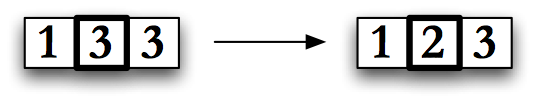
Mutation
Mutation is the process of changing an individual in a random way, Fig. Mutation. For the shortest path problem, all of the genes are an integer between \(0\) and \(\psi\), so mutation might change a randomly selected Y-value, or gene, from \(3\) to \(2\) or vice-versa. As implemented for this dissertation, mutation works on a single gene, picked randomly, and changes it to another appropriate random value. Mutation is a powerful operator because it can add diversity into a population. This can allow GA to move a population away from a local minimum in search of a global one.
If mutation is used too heavily the user will move from the genetic algorithm to a random search, on the other hand, using mutation too sparingly can allow a population to stagnate. For most of the runs discussed in this dissertation, mutation will be the chosen operation 20% of the time. This value is common in the literature, and showed reasonable diversity growth for GA in all of my simulations.
Crossover
In crossover, two parents are chosen to create a new child by combining their genetic material, [Eiben and Smith (2003)]. Often crossover treats the two parents differently, like a vector cross product crossing parent A with parent B may be different than crossing parent B with parent A. Many implementations will actually do crossover twice, creating two children instead of one, allowing each of the two parents to be parent A for one of the offspring.
When diversity is high, crossover can work like mutation to keep the population from stagnating. However, as a population loses diversity, crossover can start to become a process of combining very similar individuals. In this case, crossover can’t always add back diversity, while mutation can.
Several crossover operations are defined in the following subsections. Most of the GA runs described in this dissertation use uniform crossover as the reproduction operator \(70\%\) of the time. Unless noted, all of the runs produce two children from each crossover.
Single Point Crossover
The simplest form of crossover is single point crossover. Think of the encoded individual as a chromosome of length \(L\). Pick a random number between \(0\) and \(L\), call it \(X\). Take all of the encoded information to the left of \(X\) from one parent, and to the right of \(X\), inclusive, from the other parent. Concatenate these together to get a new child. This is single point crossover as pictured in Fig. Single Point Crossover.
Single point crossover can be restricted by the encoding scheme. For example, if individuals can only be a fixed size, single point cross over has to use the same value for \(X\) for both parents. However, if children can have a longer encoding than their parents we can choose different values of \(X\) for each parent. If the encoding requires specific groupings of genes, the crossover scheme can be customized to respect these groupings when picking \(X\).
Multipoint Crossover
Multi-point crossover, pictured in Fig. Multipoint Crossover, is similar to single point crossover, except that more than one crossover point \(X\) is selected. Like single-point crossover, there are variations that allow the genes to grow or shrink. The number of points used for crossover can range from 1, which is just single point crossover, to the total number of elements in an individual. This limit is called uniform crossover.
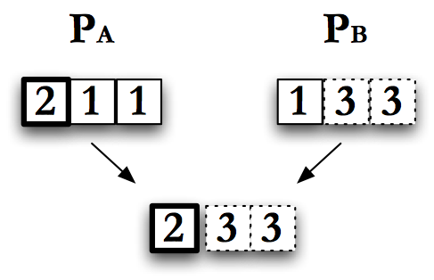
Uniform Crossover
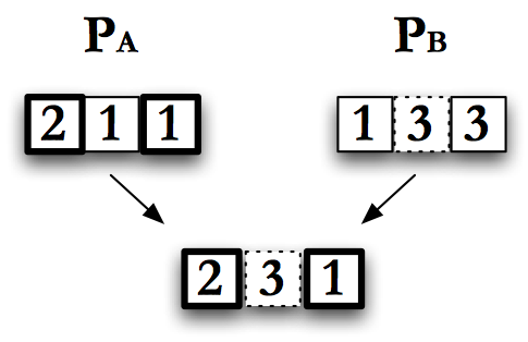
In uniform crossover, each gene of the child is selected from one parent or the other by coin-flip, at the same gene location. So, for example, if a child has \(5\) genes, numbered 1 to 5, for the first gene you randomly pick parent A or parent B and take their value for gene 1. Then you continue this process for the other 4 genes. This is the same as doing multipoint crossover with a crossover point at every gene.
Uniform crossover may appear random at first glance. But as individuals approach an optimized solution, and become more alike, the random choice between parents becomes uneventful and will produce the same gene in either case.
Many of the projects performed for this dissertation attempt to optimize geometric solutions where material is moved around in a two and three dimensional space. Uniform crossover was chosen as the main crossover type because it allows a nice random mixing of parents to create new children, see Section Single Point. Each gene for our shielding problems will represent shield material at a specific location. Uniform crossover will simply mix two shields, location by location.
Uniform crossover easily produces two children, by using parent A for the first child’s and parent B for the second child’s gene for each slot. I will use it this way throughout the dissertation.
Copy
The simplest operation in GA is copying. A parent is copied, or cloned, to create a child. Copying is especially valuable in generational GA since it allows good individuals, or bad individuals with some good genetic material, to stick around unchanged between generations. Keep in mind that this idea of keeping good genetic material is abstract, the GA itself has no concept of good versus bad material, only fitness scores to judge individuals on. Most of the optimizations discussed in this dissertation have a \(10\%\) chance of copy forward as the reproductive operator. This results in a standard break down for this dissertation of \(10\%\) copy forward, \(70\%\) crossover and \(20\%\) mutation when an operation is required.
Results for the Shortest Path Problem
Now that we have a basic understanding of what a genetic algorithm is and the standard operations, let’s take a look at how GA performs on the sample problem from Section Shortest Path Problem. We will look at the problem with two values of \(\psi\) to see how GA deals with increasing the size of the search space.
The Shortest Path Problem with \(\psi = 8\)
To start, I will set \(\psi = 8\). This means there will be \(7\) elements in the chromosome, and each element can be an integer from \(0\) to \(8\). This results in a problem space of size \(9^{7} = 4.78\times 10^6\), or about 5 million possible individuals.
The GA will use tournament selection with a tournament size of \(5\). There will be a \(25\%\) chance of the worst individual being selected in a tournament. Each new individual will be created using the following operational breakdown:
-
\(70\%\) chance of single point crossover on reproduction
-
\(20\%\) chance of mutation on reproduction
-
\(10\%\) chance of copy on reproduction
GA will run for \(40\) generations with \(2{,}500\) individuals per generation. As a result, the GA will test a total of \(100{,}000\) individuals. These individuals will not necessarily be unique, so this is an upper bound. The GA will test less than \(2\%\) of the possible solutions that use this encoding.
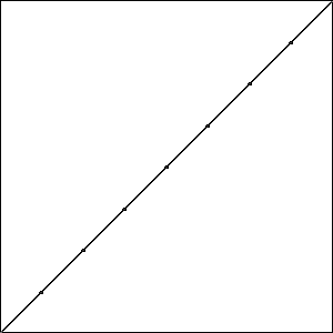
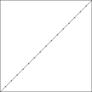
I did three runs of GA using these settings. The best possible score with \(\psi = 8\) is \(-0.414\) which is equal to one minus the length of a straight line from the origin to \((1,1)\); all three runs produced an individual that matched this score. Graphically, these three best results look like the data in Fig. Plain-Easy-Best.
To really see how well GA did, we need to look at the best fitness for each generation in one of these three runs. Graphing the fitness for the best individual in each generation versus the generation count gives the plot in Fig. Plain-Easy-MaxFit.
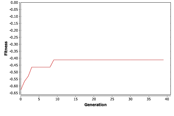
GA is finding the best solution in generation \(11\). This means that GA only needed \(27,500\) individuals to find the best solution, which is well under \(1\%\) of the total possible solutions.
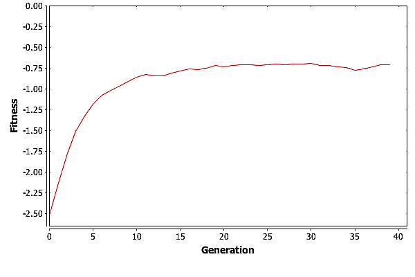
So what is GA doing after generation \(11\)? For the most part it is improving the suboptimal individuals. We can see this by looking at the average fitness by generation, pictured in Fig. Plain-Easy-AvgFit. The average fitness is going up with each generation as the good genetic material is spread around the population. Then at around \(30\) generations, GA is reaching a plateau where the average fitness is basically trapped.
Having the average fitness get trapped is not unexpected. As the population becomes more homogeneous, the only operator that really moves individuals around the solution space is mutation. Consider the simple example of a population where no individuals contain a \(0\) in their first gene. Mutation is the only way to get a \(0\) into that gene. But mutation can both hurt and help and individuals score. As the population gets closer to the best solution, or a local maximum, mutation can move it away from that maxima, and it can take numerous tries for an individual with a needed gene to participate in reproduction. In the worst case, mutation could cause the best individual in a population to score lower on the fitness function.
The Shortest Path Problem with \(\psi = 16\)
GA was able to handle a search space with five million individuals pretty easily. Let’s look at how it will do with a bigger search space. In this case, we will look at our shortest path problem with \(\psi = 16\). This is a problem space with \(17^{15} = 2.86\times10^{18}\) or \(2.86\) quintillion individuals. We will keep our GA parameters the same. The \(100,000\) individuals tested will represent only \(2.86 \times 10^{-11}\) percent of the possible solutions.
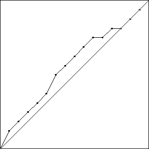
I did three runs of this problem, and all three resulted in a best fitness of \(-0.4396\) compared to the best possible fitness of \(-0.414\). While the runs all had the same best fitness score, they did not result in the same solutions. Solutions with the best fitness from each run are pictured in Fig. Best Results.
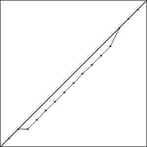
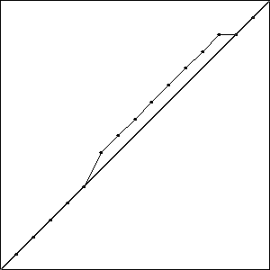
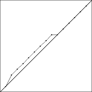
Each of these solutions is partially on the optimal line, and partially off the line by one unit, creating a bump. It is important to note that while these three individuals had the best score for their run, they are not the only individuals in that run to achieve that score.
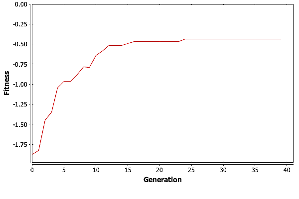
The fitness for one of these runs, pictured in Fig. Plain-Medium-MaxFit, shows that the GA is stagnating. It hasn’t had time to find a solution that can move the bump onto the line.
Consider the montage of \(25\) individuals from the last generation of Run 3, Fig. Plain-16-Montage, we can see that the population does have the genetic material needed to find the best solution. It just hasn’t found that solution yet. A few of the solutions in the montage are on the line except at the ends, while others have trouble in the middle.

The run that failed to find the best solution actually ended up with a worse solution than the runs with fewer resources. This variance demonstrates the problematic randomness of GA, while the improvement of the other two runs shows how more resources can help GA move toward a better answer. Keep in mind that while we did double the number of individuals, the number of individuals tried versus the total number of possible individuals is still miniscule.
Population Sizing and the Number of Generations
The test problem has lead us to an interesting question. How big should a population be for a given problem?
At the lower end, GA needs a population that is big enough to have sufficient diversity. For example, if we use \(\psi = 4\) and a population of \(2\) there will not be enough diversity to try to solve the problem. In order to formalize this idea of sufficient information, researchers have decomposed the Genetic Algorithm into a set of requirements. One decomposition that has been proposed, [Goldberg (1989)] , and used extensively relies on the concept of building blocks. Building blocks, [Goldberg, Deb, and Clark (1991)], are the elements that can be used to make solutions. In our sample problem the building blocks would simply be the individual points, or possibly chains of values that fall on the line that makes the best solution. Building blocks are a very abstract idea that tries to provide a concept for the useful information chunks encoded in a chromosome. In biology a building block might be the set of genes that create the heart or lungs.
The building block decomposition works like this:
-
Know what the GA is processing: building blocks
-
Ensure an adequate supply of building blocks, either initially or temporarily
-
Ensure the growth of necessary building blocks
-
Ensure the mixing of necessary building blocks
-
Encode problems that are building block tractable or can be recoded so that they are
-
Decide well among competing building blocks
The population size question address the second item of this decomposition: ensuring an adequate supply. The genetic operators like crossover and mutation ensure the growth of necessary blocks. Selection, along with the operators, ensures proper mixing. The chromosome encoding and fitness function address the last two pieces of this decomposition. We could re-write this decomposition using the terms we have been using to say:
-
Encode problems in a way that works well with mutation and crossover
-
Ensure an adequate and diverse population
-
Ensure that mutation and crossover can reach all of the genes
-
Define a good fitness function
If we consider that the initial population for GA is usually generated randomly, it is easy to see that a very small population size could prevent GA from having all of the necessary building blocks in the initial population. If this were the case, GA would have to try to use mutation to create these building blocks, which could be quite inefficient. As a result, we can theorize that given limited resources there is a population size that is too small for GA to build a solution in a reasonable amount of time.
Population sizing is bounded from above based on computing resources. While there are no papers saying that an infinite population is bad, it would require infinite resources. So as GA is applied to a problem, researchers want to find the smallest population that will still allow GA to work. Moreover, because a small population provides more opportunity for two specific individuals to crossover, small populations have the potential to evolve faster during the initial generations. Large populations, on the other hand, will have a harder time putting two specific individuals together, which can result in slower evolution.
One attack on the population sizing problem is given by Harik [G. Harik et al. (1997)]. In this paper the building blocks that represent parts of a good solution are treated as individuals that might be removed from the population via standard operators and selection, a form of gambler’s ruin. Using this concept Harik et.al. show that problems that require more building blocks are more susceptible to noise and thus more susceptible to failure. They were also able to show that while this semi-obvious connection exists it is not a scary one. The required population size for a problem is shown to grow with the square root of the size of the problem, as defined as the number of building blocks in a chromosome.
Another look at the sizing problem was done by [Goldberg, Deb, and Clark (1991)]. Goldberg et.al. used an analysis of noise in the GA to show that the required population size is \(O(l)\) where \(l\) is the length of a chromosome, or encoding. The multiplier for this equation can depend on \(\chi\), the number of possible values for each element in the chromosome, which is a fixed value for the problem.
These two analysis used different techniques to arrive at a scaling, and resulted in different values. Harik’s analysis says that the required population goes with the square root of the number of building blocks, while Goldberg’s analysis says that it increases linearly. While both analysis rely on assumptions that make them inexact, we can at least see that GA does not appear to require a population size that grows exponentially or with some power of the problem size.
On the other side of the table is the question of how many generations we should run. [Goldberg and Deb (1991)] have analyzed this problem as well to show that using standard selection mechanisms GA should converge in \(O(\log(n))\) or \(O(n \log(n))\) generations, where \(n\) is the population size. While this equation doesn’t give us an exact value for the number of generations to use, it does tell us that adding generations is not going to give us exponential improvement. It also explains the shape of the fitness graphs in Figures Plain-Easy-MaxFit and Plain-Medium-MaxFit, where we could see the slope of the fitness improvements going down with each generation.
In all of the experiments presented in this dissertation, the population sizes and generation counts have been arrived at primarily through resources constraints. I have tried to find a compromise between computing resources and reasonable results from the GA.
GA For Hard Problems
As we saw in Section Short Path Plain, even a simple problem description can result in a huge problem space. As the problem spaces get bigger, the problems get harder to solve. Hard problems can also be defined by the amount of resources they require to calculate a fitness function. In this dissertation I will be discussing problems that require radiation transport simulations to calculate a fitness score. These problems can run for minutes or hours, as opposed to the microsecond test times of the shortest path problem. As people have tried to apply GA to harder problems, they have reached a point where a single computer cannot provide sufficient resources for their problem. When this happens, the Genetic Algorithm has to be distributed to multiple computers.
Luckily, GA has an inherent parallelism. The most expensive part of GA is generally the scoring step and the process of scoring individuals can be distributed quite easily. In this section I will discuss a number of the techniques used to distribute GA onto multiple processors and machines.
Hard problems can also introduce other issues into standard GA. Sometimes diversity becomes an issue in a very large problem space. Populations can converge too quickly, or not quickly enough due to resource constraints. Some of the following techniques have been created to help change the diversity from the standard algorithm or distribute on a network, or both. These techniques are important to understand so that they can be contrasted with our new approach, MGGA.
Simple Distributed Genetic Algorithms
Perhaps the simplest way to distribute GA is to distribute the scoring phase using some form of messaging passing technology like MPI. Distributing GA using messaging passing involves running numerous agents. Most of the agents score individuals in the genetic run. A central, or master, agent performs the initial population creation, hands out scoring work, coalesces scoring results and performs reproduction. By scaling the number of agents, the scoring work can be scaled to any number of machines.
Distributed GA relies on data sharing to pass scores from the scoring workers to the scaling worker. Some form of synchronization must be provided to keep each agent doing work at the right time, and waiting while new work is created. Simple GA codes will generally use memory to hold populations, but by leveraging a shared file system, database or distributed cache, these techniques can support gigantic problems [SQLite (2011)].
Ironically, the biggest drawback of these distributed GA is that it doesn’t change the underlying algorithm. If diversity is a problem for a specific application, distributing it won’t increase the diversity. Distribution simply adds processing power. The next few sections discuss techniques that have been used to alter the fundamental algorithm. These can be combined with simple distributed Genetic Algorithms, or be distributed themselves.
Island Model Genetic Algorithms
The island model of GA, [Eby et al. (1999; Tomassini 2005)], breaks a single Genetic Algorithm run into a set of runs. Each run uses the standard iterative approach discussed in [the-ga]. What makes the island model different than running a bunch of separate GAs, is that individuals from each population, or island, are traded with other islands. So individuals from one run will migrate to, or be injected into, another run. This immigration model allows the sharing of genetic material and can add diversity by adding variety to a stagnating population.
The island model is the basis for most of the distributed algorithms used for GA by other researchers. It can be altered to allow things like different fitness functions for each island, or different GA parameters for each island. In Chapter MGGA we will see how MGGA is similar to the island model, except that we will not be performing immigration every generation or two, rather we will be using a hierarchy of populations, that could be thought of as islands. This is a the next chapter in my dissertation and i plan to post it later
Pyramidal Genetic Algorithms
In pyramidal GA, [Aickelin (2002)], a number of islands or agents are used to perform separate Genetic Algorithms. Each agent uses a different fitness function to score individuals. These individuals are then combined, or injected into a different agent that uses a higher order fitness function. For example, one agent might score a shield on mass, while another scores it on shielding quality. The final population is generated from shields that are good for mass, combined with those that are good for shielding, and GA is performed on this combination population. The final agent would use a fitness that scales for both mass and shielding.
Multiscale Genetic Algorithms
Multi-scale GA is a version of the island model where the fitness functions for each island leverage some sort of scaling in the fitness function. For example, one island might use a coarse grid, while another uses a fine grid, to score individuals, [Babbar and Minsker (2003)]. This technique is one of the motivators for MGGA. Multi-scale GA allows some of the islands to perform quick fitness tests using low resolution models, while other islands use higher resolution models to determine higher quality fitness values.
Hierarchical Genetic Algorithms
Hierarchical GA, [De Jong (2011)], is a term used for a version of the island model that is similar to Multiscale GA and Pyramidal GA. Essentially the islands form a hierarchy, where each looks for individuals based on a subset of the total criteria, and those individuals are used to feed islands looking at more criteria. Hierarchical GA has primarily been implemented as part of Genetic Programming to protect functions or other modules that have been found in the lower level islands.
Messy Genetic Algorithms
Another technique used to apply GA to hard problems is called Messy Genetic Algorithms, [Goldberg et al. (1993)]. Messy Genetic Algorithms use genes to encode name-value pairs so they can change size without breaking the standard operator semantics. The MessyGA uses a series of phases, [Merkle, Gates Jr., and Lamont (1998)], just like generational GA, but the phases are slightly different. First, there is an initialization phase. This phase is used to create all of the fundamental building blocks, but not all of the possible individuals. In our sample problem this would mean making sure that at least one individual had each of the appropriate points, but not necessarily all of the appropriate points. In a shielding problem, this might mean making sure that we have at least one individual with each part of the shield geometry included. For very large problem spaces, this rule can be reduced to simply try to create as many as the resources support.
After initialization, MessyGA uses a primordial phase composed of alternating tournament selection and building block filtering (BBF). The tournament selection finds fit individuals, and BBF deletes genes. Individuals that can have genes deleted and are still highly fit are passed into the next phase. The next phase is called juxtaposition. In this phase, individuals are recombined to build better individuals. These phases are often distributed across multiple machines.
Messy GA focuses on the building block concept by trying to ensure that all of the good building blocks are available and that these building blocks are highlighted and combined into highly fit individuals. Messy GA has been written in a highly parallel fashion to support hard problems and its building block nature helps it focus on preserving good building blocks even in limited populations.
Genetic Algorithms on an Off-The-Shelf Cluster Scheduler
The problems discussed later in this dissertation are “hard problems." They have large solution spaces, and they require a lot of computing resources to score. Luckily a large cluster is available at the University of Michigan. This section discusses why I developed a genetic algorithm library to execute GA on the U of M cluster.
The U of M cluster uses the Portable Batch System (PBS) scheduler, see [ (Anon. 2011)]. This is a very standard, open source, cluster job scheduler. In order to put GA onto the Michigan cluster and scheduler I had to stay within a set of restrictions.
-
All jobs for a genetic run must be scheduled in advance.
-
Jobs must be assigned an estimated time.
-
Jobs are only given their estimated time to complete, plus a margin for error.
-
Jobs that run over their time, plus the margin, are treated as failed and killed.
-
The longer the estimated time for a job, the lower priority it has.
-
Jobs can depend on one or more other jobs, in a flexible manner.
-
There is a line length associated with listing dependencies.
-
My jobs running on another user’s nodes can be interrupted.
-
Jobs have access to a shared file system.
Estimating time, dealing with errors for fault tolerance and working around line length limits are the main issues with leveraging the existing cluster. Moreover, in order to scavenge the most resources, my code had to be resilient to interruptions. The PBS scheduler doesn’t like to schedule many long running jobs for a single user on shared computers. Having long running jobs reduced our resource usage by reducing our priority. Finally, the cluster administrators didn’t want my jobs to schedule other jobs to solve this problem.
Considering these restrictions I decided to leverage the PBS scheduler as the master node and use the job running nodes as the scoring slaves in a distributed GA. In order meet the restrictions I also replaced the message passing design with a batch design. Instead of agents running all of the time, a series of jobs is scheduled for each phase in the GA process. For example, a job builds the initial population, a set of jobs score the population, a job processes the scores, a job performs reproduction, etc.. As with the message passing design, batch distributed GA can be scaled to fill available computing resources. Unfortunately, there are no GA libraries, that I could find, that support the concept of the batch-oriented distributed GA on this type of job scheduler, with my resource restrictions. As a result, I implemented batch distributed GA in a custom library called Genetik. Genetik is avaialble on github.
I was unable to find any reference to this style of distributed GA in the literature and as a result, this implementation of batch GA in the context of a job scheduler appears to be a new technique.
Generational GA As Jobs
Genetik uses the following basic job types to do the actual work:
Build : Build a population, either randomly or from a previous one.
Score : Score a sub-set of a population.
Collect And Scale : Join the scored sub-sets and perform any fitness score scaling we want to do.
The input file for Genetik includes how many individuals should be included in each generation and how many generations to increment over. Genetik uses this information to schedule one build job for each generation and one collect and scale job for each generation. The input file also contains the size of the scoring populations. Genetik uses this information to schedule enough scoring jobs to cover the population.
The build job uses a cache of all previously scored individuals to ensure that no individual is scored in two different generations. It is possible that the same individual is scored by 2 scoring jobs, but it will not be scored again in a later generation.
The genetik input file also contains time estimates for each job type. These are included in the PBS job description files.
Dealing with Dependency Limits
PBS has a line length limit for describing dependencies. This restriction is at odds with our desire to scavenge as many computing resources as possible. In order to scavenge all possible resources we want to run a lot of short running jobs, rather than a few long running jobs. Having a lot of scoring jobs for each generation places a long dependency list on the Collect and Scale job that follows them. In order to coalesce these dependencies into reasonable line lengths, I use no-op jobs called Joins. These jobs do nothing, but do have dependencies. Using a 5-to-1 scaling I can quickly reduce a large number of scoring jobs into a small number of Join jobs that can be depended on by the Collect job.
Dealing with Errors
Scoring jobs can fail; the easiest way this can happen is if we underestimate the time it takes to score an individual. I have built in some resilience against scoring jobs failing. This resilience comes in the form of a repair step in the collection process. Repairs simply replace an individual that couldn’t be scored with a random, scored, individual.[^1]
Processing
The final step in my implementation of GA on the PBS scheduler was to add pre-processing and post-processing jobs. These jobs allow different runs to initialize data sets, and to build reports. Also, the standard post processing step cleans up the PBS job descriptions.
These two new jobs, along with the others I have described result in the following mapping of GA onto the PBS scheduler.
Pre-Process : Perform any initialization.
Build : Build a population, either randomly or from a previous one.
Score : Score a sub-set of a population by running a radiation transport code multiple times.
Join : Join scoring jobs, treated as dependency lists, into 4 or fewer dependencies.
Collect And Scale : Make sure that the scoring jobs worked, and if not replace individuals that didn’t get scored with random copies from their parent generation. Join the scored sub-sets and perform any scaling we want to do.
Post-Process : Build a report of the results and clean up unneeded files.
To iterate over generations, I unroll the loops associated with generational GA. This design has been tested with numerous runs on the Michigan cluster called NYX and provides good cluster usage, some runs used over \(40\) machines across several hundred jobs.
Genetik On A Proprietary Cluster
For parts of this dissertation, funded by a grant, I was able to reserve time on the U of M cluster. This allowed me to move to a single job that ran GA and used an MPI version of MNCP to leverage the clusters computing resources. This single job model is not unique and is very powerful, but was only available after I obtained reserved computing resources, so that my single jobs could run for days. This type of long running job would not work when I was scavenging resources. The single large job with MPI-based MCNP performed similarly to the batch model, but was easier for the cluster administrators to support.
Optimizing GA
The Genetik library included two mechanisms to try to reduce fitness function executions, caching and pre-calculating. These two methods optimize the time spent on the cluster.
Caching involves remembering or at least checking the scores of individuals against the fitness functions that have already been run before executing their fitness function. On a very fast problem, like the shortest path, this is not very useful. But for the problems discussed in this dissertation where a fitness evaluation can take more than ten minutes, the time spent building and checking a cache becomes a very good investment. Genetik builds a cache from previous generations before scoring the next generation. This cache maps the chromosome for an individual to a score. By caching in this way, GA can save scoring time even if an individual disappears from the population and reappears in a later generation.
When Genetik was being written I had a novel idea that we could pre-determine all of the work we would have to do before we start running. Using this information, we could eliminate fitness function executions by finding individuals that never reproduce and not scoring them. I implemented this concept, called pre-calculation, by building a plan for each generation that included which individuals would be chosen with selection, which were mutated, which were copied and which participated in crossover to create the next generation. By finding which individuals were never chosen I was able to avoid scoring them. This method does not actually know which individuals will exist, it depends on indices into the population. So the plan might say, perform a tournament on 1,5,20,54 and 100 and create a child by mutating the winner. We don’t know which will win, but we do know that we need to score the individuals at those five indices in the population to run the tournament.
The first version of Genetik implemented pre-calculation, but it turned out that very few individuals were skipped. This is a good thing. Tournament selection does a very good job of allowing almost every individual to participate in tournaments. So almost every individual at least has a chance to reproduce. While pre-calculation appears to be a novel idea, and I was unable to find it in any prior work, it doesn’t appear to be an incredibly useful idea, so I removed it from the second version of Genetik, greatly simplifying the code.
Summary
Genetic Algorithms are a very powerful technique for finding solutions to hard problems. Using a few standard operators, GA is able to find solutions in huge search spaces without examining the entire space. Solutions are assigned a value using a fitness function. Execution of the fitness functions can be distributed allowing GA to work in parallel, making it even more powerful. Using the cluster at the University of Michigan I was able to build an implementation of GA that would run in a batch mode and take advantage of free computing resources.
References
Aickelin, Uwe. 2002. “Partnering strategies for fitness evaluation in a pyramidal evolutionary algorithm.” In Proc. Genetic and Evolutionary Comput. Conf. GECCO’02, 263–270.
Anon. 2011. “PBS User Guide.” http://www.doesciencegrid.org/public/pbs/.
Anon. “babbar-mmp not found!”
Babbar, Meghna, and Barbara Minsker. 2003. “Multiscale Strategies for Solving Water Resources Management Problems with Genetic Algorithms.” In Environmental & Water Resources Institute (EWRI) World Water & Environmental Resources Congress 2003 & Related Symposia.
Banzhal, Wolfgang, Peter Nordin, Robert E. Keller, and Frank D. Francone. 1998. Genetic Programming - An Introduction. Morgan Kauffman.
De Jong, E. 2011. “Hierarchical Genetic Algorithms.” http://citeseer.ist.psu.edu/705095.html.
Eby, David, R. C. Averill, William F. Punch, III, and Erik D. Goodman. 1999. “Optimal design of flywheels using an injection island Genetic Algorithm.” Artif. Intell. Eng. Des. Anal. Manuf. 13 (5): 327–340. doi:http://dx.doi.org/10.1017/S0890060499135066.
Eiben, A. E., and J. E. Smith. 2003. An Introduction to Evolutionary Computing. Springer-Verlag.
Goldberg, David E. 1989. Genetic Algorithms in Search, Optimization and Machine Learning. Boston, MA, USA: Addison-Wesley Longman Publishing Co., Inc.
Goldberg, David E., Kalyanmoy Deb, Hillol Kargupta, and Georges Harik. 1993. “Rapid, Accurate Optimization of Difficult Problems Using Fast Messy Genetic Algorithms.” In Proceedings of the Fifth International Conference on Genetic Algorithms, 56–64. Morgan Kaufmann.
Goldberg, David E., Kalyanmoy Deb, and James H. Clark. 1991. “Genetic Algorithms, Noise, and the Sizing of Populations.” COMPLEX SYSTEMS 6: 333–362.
Goldberg, David E., and Kalyanmoy Deb. 1991. “A comparative analysis of selection schemes used in Genetic Algorithms.” In Foundations of Genetic Algorithms, 69–93. Morgan Kaufmann.
Harik, George, David E. Goldberg, Erick Cantu-Paz, and Brad L. Miller. 1997. “The Gambler’s Ruin Problem, Genetic Algorithms, and the Sizing of Populations.” In Evolutionary Computation, 7–12. IEEE Press.
Holland, John H. 1975. Adaptation in Natural and Artifical Systems. MIT Press.
Jong, Kenneth A. De. 2006. Evolutionary Computation. MIT Press.
Langon, William B., and Riccardo Poli. 2002. Foundations of Genetic Programming. Springer-Verlag.
Merkle, Laurence D., George H. Gates Jr., and Gary B. Lamont. 1998. “Scalability of an MPI-based fast messy Genetic Algorithm.” In SAC ’98: Proceedings of the 1998 ACM symposium on Applied Computing, 386–393. New York, NY, USA: ACM.
Mitchel, Melanie. 1998. An Introduction to Genetic Algorithms. MIT Press.
SQLite. 2011. “Limits in SQLite.” http://www.sqlite.org/limits.html.
Tomassini, Marco. 2005. Spatially Structured Evolutionary Algorithms. Springer-Verlag.
[^1]: I only take scored individuals for repairs, to insure that failed scoring jobs aren’t propagated to the next generation.